모델링을 위한 데이터 분석 방법 비교: simple Euler integration, Runge-Kutta 4th order
포스트 난이도: HOO_Middle
# 모델링을 위한 데이터 분석
이전 포스트, "모델링을 위한 데이터 분석",에서 4가지 계산식을 통해 산출된 결괏값들이 각기 달라질 수 있다는 걸 확인했다. 이번 포스트에서는 각기 다른 계산식일지라도 주어진 조건 값을 조정해 줌으로써 산출 결과를 동일하게 만들어줄 수 있음을 살펴볼 예정이다. 앞선 포스트에 대한 내용이 궁금하다면 아래의 링크를 통해 해당 포스트를 살펴볼 수 있다.
https://whoishoo.tistory.com/655
[Python Example] 모델링을 위한 데이터 분석 방법 Analytical solution, simple Euler integration, improved Euler integ
모델링을 위한 데이터 분석 방법 Analytical solution, simple Euler integration, improved Euler integration, Runge-kutta 4th order: #matplotlib, #for_loop, #numpy 포스트 난이도: HOO_Middle # 계산식에 따른 산출값의 변화 Timeserie
whoishoo.tistory.com
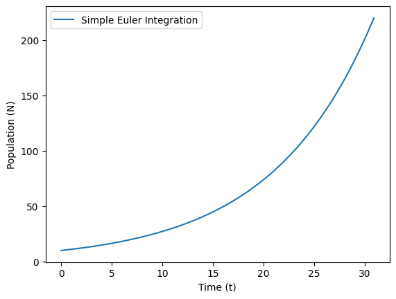
# Simple Euler integration vs RK4
실제 값과 모델링으로 나온 결과값의 차이가 발생하지만 모델링하는 과정에서 어떤 계산식이나 알고리즘을 사용했냐에 따라서도 결괏값들이 각기 다르다. 마치 우리가 자연재해를 예측하는 예보를 확인해 보면 각 모델별로 조금씩 다른 차이가 나타나는 걸 알 수 있는데, 이 역시도 모델링에 적용된 각기 다른 요소들이 영향을 주어 최종 산출되는 값이 달라지는 것이다. 앞선 포스트에서 다뤘던 Simple Euler integration과 RK4의 예제코드를 통해서 두 예제코드의 결괏값이 같게끔 조정해 보았다. 여기서 조정된 값은 델타 값만 가지고 조정이 이루어졌으며, RK4의 산출값과 동일하게 만들어주기 위해 Simple Euler integration 코드가 수정된 걸 확인할 수 있다.
#4th-order runge
import numpy as np
import matplotlib.pyplot as plt

# Constants
N0 = 10
k = 0.10
t_values = np.arange(0, 31, 0.1)
delta_t = 0.1

# 4th-Order Runge-Kutta Method
N_rk4 = [N0]
for t in t_values[1:]:
    k1 = k * N_rk4[-1]
    k2 = k * (N_rk4[-1] + 0.5 * delta_t * k1)
    k3 = k * (N_rk4[-1] + 0.5 * delta_t * k2)
    k4 = k * (N_rk4[-1] + delta_t * k3)
    N_next = N_rk4[-1] + (delta_t / 6) * (k1 + 2 * k2 + 2 * k3 + k4)
    N_rk4.append(N_next)

#Table values
for t, N_t in zip(t_values, N_rk4):
  print("time: " ,t, "/ N_t: " ,N_t)

# Plotting
plt.plot(t_values, N_rk4, label="4th-Order Runge-Kutta")
plt.xlabel("Time (t)")
plt.ylabel("Population (N)")
plt.legend()
plt.show()
#the simple Euler integration
import numpy as np
import matplotlib.pyplot as plt

# Constants
N0 = 10
k = 0.10
t_values = np.arange(0, 31, 0.1)
delta_t = 0.1005016699

# Simple Euler Integration
N_simple_euler = [N0]
for t in t_values[1:]:
    N_next = N_simple_euler[-1] + delta_t * k * N_simple_euler[-1]
    N_simple_euler.append(N_next)

# Plotting
print(N_simple_euler)
plt.plot(t_values, N_simple_euler, label="Simple Euler Integration")
plt.xlabel("Time (t)")
plt.ylabel("Population (N)")
plt.legend()
plt.show()
# github link
https://github.com/WhoisHOO/HOOAI/blob/main/Python%20Examples/runge-kutta_4th_order
https://github.com/WhoisHOO/HOOAI/blob/main/Python%20Examples/simple_euler_integration


댓글